Bayesian decision making for multi-armed bandit - Simulation example
Introduction
This example simulates a large mailing to 200,000 people. The message includes some
action that the recipients can do - or not. So for each message that is sent and received there is a probability of success or failure. We do not know this value
at the start.
The result can only be one of these options, either success or failure. In order to make the message attractive and increase the likelihood
of success it has been decided to try 10 different minor variations on the theme. This is why it is sometimes called a multi-armed bandit test - like a row of
slot machines where we do not know the probability of success for each one. Which arm should we pull next?
So the simplest way to do this test is to send 1/10 of the
total number of messages of each type; 20,000 messages for each variation in the test. At the end of the test we can sum up the total numbers of successes for each
batch and use standard statistical methods to decide which variant is most likely the best. We could use smaller batches and attempt a decision earlier. The sensitivity of our test will be determined by
the numbers chosen in each batch, we need enough to be able to definitely make a choice, but not too many that we waste effort sending to the worse choices.
This batch number will be chosen at the start and an educated guess made as to the best number to use. The Bayesian plan would be different. In Bayesian
Sequential Decision Making we do a small test, see what the evidence provides, and then use this evidence in our next small batch. So if we see a definite
pattern emerging early on, we use this evidence to moderate our choices in the future. This has the advantage of not wasting any effort on definitely poorer
chances, but also means we concentrate more effort on deciding exactly which choice is best using all the information we have to hand.
Method
Here I use the methods outlined in McInerney, Roberts and Rezek's paper of 2010 at AAMAS Workshop
on Multi-agent Sequential Decision Making entitled: Sequential Bayesian Decision Making for Multi-Armed Bandit.
Available here as pdf. I have used Matlab
(Mathworks)
to do the programming. I tested 3 scenarios; 1) a single variant with a constant batch size, to illustrate how the methods works,
2) The full simulation of 10 iterations of 20,000 spread between 10 variants, and,
3) A default test of 20,000 to each of the 10 variants without the Bayesian sequential decision making to contrast the results.
The steps for the simulation, scenario 2 above, are as follows:
Results
Scenario 1: single variant and constant batch size.
Here I used a constant batch size and a single test variant to see how the beta
distribution progressively estimated the value of the hidden variable.
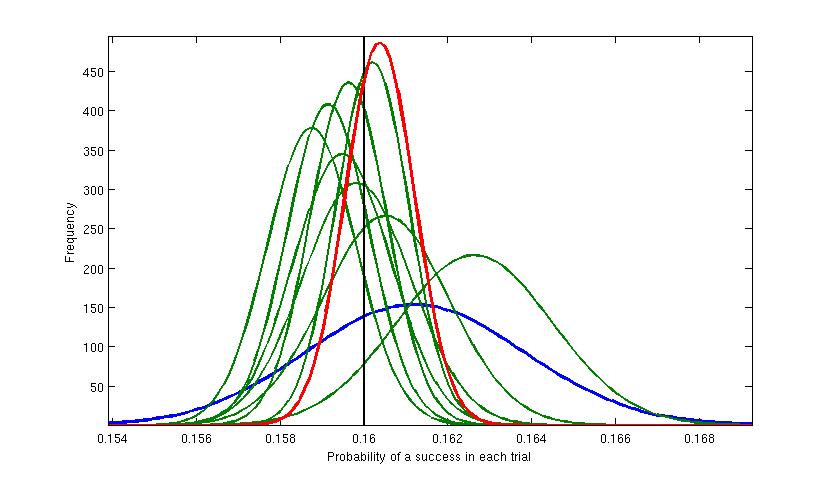
Figure 1. Here a single test variant was used and at each iteration the sending of 20,000 test messages was simulated. The vertical black line shows the value of the
hidden variable that was used to generate the results. The first batch of 20,000 returned around 3230 successful responses. This was modelled
with a Beta distribution shown by the blue curve. This is the widest and thus least accurate estimate for the true value, illustrating our relative high uncertainty at
this stage. The mean value for
this Beta distribution is about 0.1615 (value of the highest point), which is an estimate of the true value (0.16). Then at each iteration (the green curves) the distribution
gets slimmer (more accurate) and generally closer to the true value. Each new model is using the previous result as the prior probability distribtuion and
moderating it using the new evidence - using Bayes Theorem. The final iteration is represented by the red curve and estimates the true value at around 0.1605.
Main test, scenario 2.
For the main test of 10 different variants I used the following hidden probabilities:
16, 24, 29, 30, 22, 30.3, 23.5, 26, 30.6, 21
These are percentage chances of a success from each of the test variants. So variant #9 had the highest chance of success, but #4 and #6 were very close to #9.
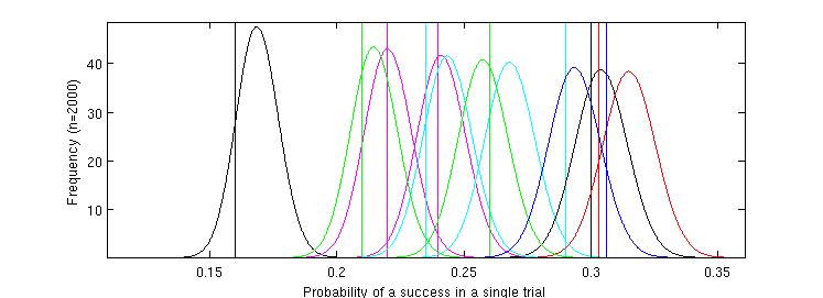
Figure 2. The probability density functions of the beta distributions modelled from the first batch of 2000 messages of each type.
This information is used by the program automatically as it steps through the process but shown here for illustration. Each
curve relates to a different test variant. The values of the true (but hidden) probabilities for each variant of the test message are shown as vertical lines.
Each curve roughly coincides with the value of the hidden probabilities but the figure demonstrates that accurate differentiation between some of the hidden variables
is not possible with this information. This is especially true of the highest values - the test has been set up to explore this type of problem. The worst
variants are visible toward the left of the figure and there is clear space between the curves for these and the more successful ones.
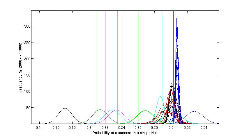
Figure 3. A full simulation run of 200,000 messages over 10 iterations. This graph shows that the method has ignored the worst variants, and the position
for each of these is similar to that shown in Figure 2. No further simulated messages have been sent using those variants. All the action is at the other
end of the graph around the variants which have shown to be probably best. The blue red and green sets of curves on the right hand side of the figure.
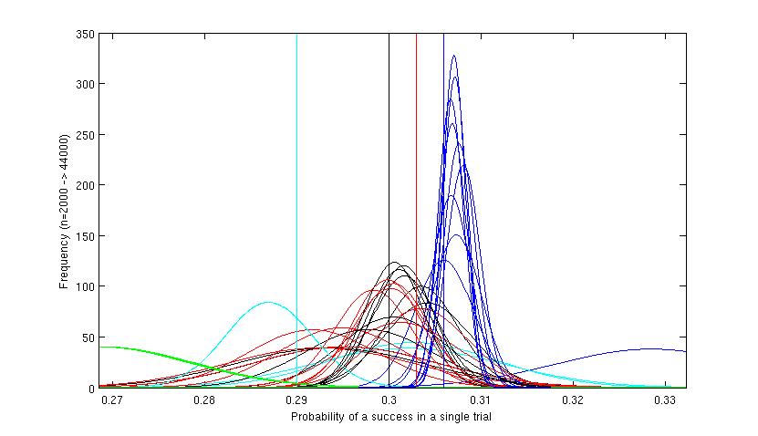
Figure 4. Detail of upper end of Figure 3. Here the separate curves for the iterations at the higher levels can be seen. The extreme right hand curve shows
the first rather inaccurate estimate for the most successful (blue) variant. The figure shows that the program has concentrated around the black, red and blue
variants, and has eventually 'homed in' on the blue and the final few iterations were concentrated almost exclusively on this variant, which by that time
could be reliably determined as the best. The cyan (light blue) variant had looked promising at first but has been 'tested out' after its cumulative results
proved that it was in fact not the best variant. The green had been tested a few times before being discarded. The red and black did not have enough tests to differentiate
between them, but although they continue to be tested throughout the scenario, by far the greatest effort is directed at the blue variant and evidence accrues
that it is probably the best variant.
Numerical results: Standard test using 10 iterations of 20,000:
Default method: scenario 3 using a single iteration of 200,000 spread evenly:
Summary of results
The overall success rate of the Bayesian sequential decision system is higher (roughly 30% success as opposed to 25%). This is because the method
avoids wasted effort on the least well performing variants. The final probability estimate that the best single variant is identified is higher with the Bayesian system.
This is because more effort is concentrated on the more successful group of variants which provides higher sensitivity to differentiate them.
Discussion
Seems to work reasonably well. Drinks all round.